电路用于给电容器和电感器充电。然后将电感器/电容器从充电电路切换到放电电路。有三个概念
- 充电电路... 假设在很长一段时间内... 假设稳态,所以电容器是开路,电感器是短路
- 切换电路(电容器和电感器的不同)
- 放电电路... 假设电容器最初是短路,电感器是开路
有两个电路需要分析:充电和放电
- 充电电路... 假设初始条件为零,求稳态(特解)... 这些成为放电电路的初始条件。
- 放电电路求解(齐次解)。
求解放电电路有以下步骤
- 假设解是指数函数
- 找到一个指数解
- 利用初始条件和最终值条件求解常数。
- 如果能找到指数解(即存在实部),则假设有效。
-
由开关隔开的电容器充电和放电电路
-
等效充电电路
-
大多数开关是
BBM(断开后再闭合),因此电容器在单极切换到两个极之间时是开路。
超级电容 存储大量能量,充电速度非常快,放电速度非常快,可以替代电池。
-
等效放电电路
充电分析是稳态分析。假设电路已经运行了很长时间。电容器已经有了足够的时间充电。
不同之处在于,这里不是正弦波电源,而是直流电源。电容器上会有一个直流稳态电压。
电容器在完全充电时看起来像一个开路,因此整个电源电压将出现在电容器上。因此在这种情况下,电容器上的初始电压为 1 伏。
 观察电容器放电,标记电流方向和电压极性,使其与华夏公益教科书电路理论的正常端子关系一致。
一个简单的网格或回路分析(两者都会得出相同的方程)是


从电容器端子关系

所以代入

当然,经过很长一段时间,电容器放电,电阻耗散掉所有能量,所有地方的电流和电压都将为零。但是,描述电压和电流如何趋于零的时域方程是什么?
请注意,电流在充电时正在下降,但在放电时切换到上升。这可能是瞬时的。
一般技术是假设这种形式

代入上述微分方程

除以 A 和指数函数,得到

求解 tau

因此,电容器两端的电压公式现在是

这包括 0 的稳态特解和来自求解微分方程的常数 C。
电容器两端的初始电压在 t=0+ 时为 +1 伏。这意味着

经过很长一段时间,V_c(t) = 0。这有助于我们找到 C

所以 C = 0 且 A = 1,并且

观察电容器放电,标记电流方向和电压极性,使其与华夏公益教科书电路理论的正常端子关系一致。
Vc=-Vr 或者可以代入电容器端子关系

因此对于此电路


并且

Vc 处于指示的极性。VR 与所绘制的极性相反。电流流向与所绘制的方向相反,这在电容器充当电压源并将能量倾倒到电阻器时是有道理的。两者在 5 个时间常数 (50 μs) 后将基本为零。
齐次解很容易找到,因为使用直流电源来为电路充电。放电电路的特解为 0,因为没有激励函数。
 当电感器具有与电流源相同的初始电流时,就不会有电流流过短路。叠加原理表明电流将在短路中抵消。
充电分析是稳态分析。假设电路已经运行了很长时间。电感器有足够的时间建立其磁场。
不同之处在于,使用直流电流源代替正弦波源。电感器中将会有一个直流稳态电流。
电感器在完全充电时看起来像一个短路,因此整个源电流都流过电感器。因此,在这种情况下,初始电流为 1 安培。
 电感将能量存储在磁场中,电流必须持续流动以防止磁场崩溃...... 这是超导体的基础。
 具有初始电流的电感通过电阻放电,用于华夏公益教科书电路理论。
通过按下 SW1 的按钮,将电感和电流源短路是安全的。(打开连接到电感或电流源的导线是危险的)。对于理想元件,短路将没有电流。然而,通过电感的电流保持不变,电感保持充电状态。
当 SPDT 开关切断电流源时,电感的电流出现在短路中。电感和短路线不会长时间存储能量(除非冻结,因为导线充当电阻)。
在 SW2 完成切换到第二个极点并释放按钮开关后,1 安培的电流仍然流过电感。电压瞬间出现在电感和电阻之间。一个简单的网格或回路分析(两者都产生相同的方程式)将是

观察电路标记,电流和电压没有正号约定关系,因此电感的端子关系有一个负号

所以

当然,经过很长时间,电感放电,电阻耗散所有能量,并且处处电流和电压都将为零。但是,描述电压和电流如何变为零的时间域方程式是什么?
请注意,电压在电感顶部为正,但在放电时会改变极性。这可以是瞬间的。
一般技术是假设这种形式

代入上述微分方程

除以 A,然后计算导数,得到

除以指数

求解 tau

因此,电流的公式现在是

稳态特解为 0,常数 C 来自求解微分方程。
初始电流为 1 安培,时间为 t=0+。这意味着

经过很长时间,电路中没有任何活动,因此

所以 A=1 且 C=0,因此

VL=Vr 或者可以代入电感器端子关系式

或者代入端子关系式

所以总结一下


为了保持电感器的电流和磁场能量,需要在电路之间切换时将其短路。这与电容的切换一样简单,但需要不同类型的开关:…闭合前断开开关…这样两个电路就可以同时连接。
放电电路用最终方向和极性标记。但电感器的端子关系式必须有一个负号,因为电压和电流方向不符合正号惯例。
同样,齐次解很容易找到,因为使用直流电源为电路充电。放电电路的特解为0,因为没有强迫函数。

 由开关隔开的电容器充电和放电电路
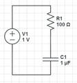 等效充电电路
 等效放电电路


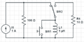 此电路显示了一个电感器置于充电电路和放电电路之间。因为大多数开关都是 BBM,所以添加了一个按钮来在投掷 SPDT 开关之前短路电感器。两个开关都可以用单个 SPDT MBB 开关替换。但是模拟软件通常只有 BBM 开关。
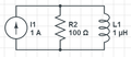 等效电感器充电电路
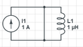 按下按钮开关后但投掷 SPDT BBM 开关之前,等效电路。
 投掷 SPDT BBM 开关时,按钮开关保持接触,等效电路。 超导体 可以像超级电容器一样充当储能装置。电流以光速通过充当连续电感器的圆形导线移动。
 释放按钮开关后,等效电感器放电电路。


