电路理论/二阶解

== 二阶解

本页将讨论二阶 RLC 电路的解。二阶解相当复杂，要完全理解它需要了解微分方程。本书不需要你了解微分方程，因此我们将描述解，而不会展示如何推导它们。推导可能会被放在另一章中，最终。

本章的目的是推导二阶电路的完全响应。确定完全响应涉及许多步骤

1. 获得电路的微分方程
2. 确定谐振频率和阻尼比
3. 获得电路的特征方程
4. 求解特征方程的根
5. 求解自然响应
6. 求解强迫响应
7. 求解完全响应

我们将逐一讨论所有这些步骤。

求解微分方程

二阶电路只有在获得描述电路的二阶微分方程后才能求解。我们将在这里讨论一些用于获得 RLC 电路二阶微分方程的技术。

注意

并联 RLC 电路使用电压的常微分方程更容易求解（基尔霍夫电压定律的结果），串联 RLC 电路使用电流的常微分方程更容易求解（基尔霍夫电流定律的结果）。

直接法

求解电路微分方程最直接的方法是对电路进行节点分析或网孔电流分析，然后求解输入函数的方程。最终方程应该只包含导数，不包含积分。

变量法

如果我们创建两个变量 g 和 h，我们可以用它们创建一个二阶微分方程。首先，我们将 g 和 h 设置为电感电流、电容电压或两者。接下来，我们创建一个只有一个一阶微分方程，它有 g = f(g, h)。然后，我们写另一个一阶微分方程，其形式为

${\frac {dh}{dt}}=Kg$ 或 ${\frac {1}{K}}{\frac {dh}{dt}}=g$

接下来，我们将第二个方程代入第一个方程，我们就得到一个二阶方程。

零输入响应

电路的零输入响应是指当没有激励函数（没有电流输入，也没有电压输入）时电路的状态。我们可以将微分方程设置为

${{d^{2}i} \over {dt^{2}}}+2\zeta {{di} \over {dt}}+\omega _{o}^{2}i(t)=0$

这导致了电路的特征方程，将在下面解释。

特征方程

RLC 电路的特征方程使用下面描述的“算子法”获得，其中输入为零。RLC 电路（串联或并联）的特征方程将是

$s^{2}i+{R \over L}si+{1 \over {LC}}i=0$

特征方程的根是我们正在寻找的“解”。

求解特征方程

这种获得特征方程的方法需要一点技巧。首先，我们创建一个算子 s，使得

$sx={\frac {dx}{dt}}$

此外，我们可以将高阶算子表示为

$s^{2}x={\frac {d^{2}x}{dt^{2}}}$

其中 x 是电路源的电压（在串联电路中）或电流（在并联电路中）。我们为电路中的电感电流和/或电容电压编写 2 个一阶微分方程。我们将所有微分转换为 s，并将所有积分（如果有）转换为 (1/s)。然后我们可以使用克莱姆法则求解。

解

特征方程的解用谐振频率和阻尼比表示

[特征方程解]

$s=-\zeta \pm {\sqrt {\zeta ^{2}-\omega _{o}^{2}}}$

如果这两个值中的任何一个都用于假设解中的s $x=Ae^{st}$并且该解完成了微分方程，那么它可以被认为是一个有效的解。我们将在下面进一步讨论这一点。

阻尼

电路的解取决于电路表现出的阻尼类型，这由阻尼比与谐振频率之间的关系决定。不同的阻尼类型包括过阻尼、欠阻尼和临界阻尼。

过阻尼

RLC 串联过阻尼响应

当满足以下条件时，电路称为过阻尼

$\zeta >\omega _{0}$

在这种情况下，特征方程的解是两个不同的正数，由以下公式给出

$I(t)=Ae^{\ s_{1}t}+Be^{\ s_{2}t}$，其中

$s_{1},s_{2}=-\zeta \pm {\sqrt {\zeta ^{2}-\omega _{0}^{2}}}$

在并联电路中

$\zeta =1/(2RC)$

$\omega _{0}=1/{\sqrt {(LC)}}$

在串联电路中

$\zeta =R/(2L)$

$\omega _{0}=1/{\sqrt {(LC)}}$

过阻尼电路的特点是稳定时间很长，并且可能存在较大的稳态误差。

欠阻尼

当阻尼比小于谐振频率时，电路称为欠阻尼。

$\zeta <\omega _{0}$

在这种情况下，特征多项式的解是共轭复数。这会导致电路中出现振荡或振铃。该解包含两个共轭根

$\lambda _{1}=-\zeta +i\omega _{c}$

和

$\lambda _{2}=-\zeta -i\omega _{c}$

其中

$\omega _{c}={\sqrt {-(\omega _{o}^{2}-\zeta ^{2})}}$

该解决方案是

$i(t)=Ae^{(-\zeta +i\omega _{c})t}+Be^{(-\zeta -i\omega _{c})t}$

其中 A 和 B 是任意常数。使用欧拉公式，我们可以将解简化为

$i(t)=e^{-\zeta t}\left[C\sin(\omega _{c}t)+D\cos(\omega _{c}t)\right]$

其中 C 和 D 是任意常数。这些解的特点是 指数衰减的正弦响应。品质因数（见下文）越高，振荡衰减所需的时间就越长。

临界阻尼

RLC 串联临界阻尼

如果阻尼系数或实际阻尼与临界阻尼之比等于 1，则电路称为 临界阻尼

$\zeta =1$

在这种情况下，特征方程的解是二重根。两个根是相同的（$\lambda _{1}=\lambda _{2}=\lambda$），解为

$I(t)=(A+Bt)e^{\lambda t}$

其中 A 和 B 是任意常数。临界阻尼电路通常具有较低的过冲、没有振荡和较快的稳定时间。

串联 RLC

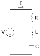一个串联 RLC 电路。

具有恒定电压源 V 和电阻 R、电容 C 和电感 L 的简单串联电路的微分方程为

$L{\frac {d^{2}q}{dt^{2}}}+R{\frac {dq}{dt}}+{1 \over C}q=0$

因此，特征方程如下

$Ls^{2}+Rs+{1 \over C}=0$

有两个根

$s_{1}=-{R \over 2L}+{\sqrt {({R \over 2L})^{2}-{1 \over LC}}}$

和

$s_{2}=-{R \over 2L}-{\sqrt {({R \over 2L})^{2}-{1 \over LC}}}$

并联 RLC

一个并联 RLC 电路。

具有电阻 R、电容 C 和电感 L 的并联 RLC 电路的微分方程如下

$C{\frac {d^{2}v}{dt^{2}}}+{\frac {1}{R}}{\frac {dv}{dt}}+{1 \over L}v=0$

其中 v 是电路上的电压。因此，特征方程如下

$Cs^{2}+{1 \over R}s+{1 \over L}=0$

有两个根

$s_{1}=-{1 \over 2RC}+{\sqrt {({1 \over 2RC})^{2}-{1 \over LC}}}$

和

$s_{2}=-{1 \over 2RC}-{\sqrt {({1 \over 2RC})^{2}-{1 \over LC}}}$

电路响应

一旦我们得到了微分方程和特征方程，我们就可以组装电路响应的数学形式。RLC电路的微分方程形式为

$a_{2}{\frac {d^{2}x}{dt^{2}}}+a_{1}{\frac {dx}{dt}}+a_{0}x=f(t)$

其中f(t)是RLC电路的激励函数。

自然响应

电路的自然响应是指给定电路对零输入的响应（即仅取决于初始条件值）。电路的自然响应将记为x_n(t)。系统的自然响应必须满足电路的无激励微分方程

[无激励函数]

$a_{2}{\frac {d^{2}x}{dt^{2}}}+a_{1}{\frac {dx}{dt}}+a_{0}x=0$

我们记得这个方程是上面讨论的“零输入响应”。现在我们定义自然响应为指数函数

$x_{n}=A_{1}e^{st}+A_{2}e^{st}$

其中s是电路特征方程的根。选择x_n的这个特定解的原因是基于微分方程理论，我们将暂时不加证明地接受它。我们可以使用两个方程组来求解常数值

$x(0)=A_{1}+A_{2}$

${\frac {dx(0)}{dt}}=s_{1}A_{1}+s_{2}A_{2}$

其中x是电压（在并联电路中的元件）或电流（在串联电路中的元件）。

强迫响应

电路的强迫响应是指电路对输入激励函数的响应方式。强迫响应记为x_f(t)。

其中强迫响应必须满足强迫微分方程

[强迫函数]

$a_{2}{\frac {d^{2}x}{dt^{2}}}+a_{1}{\frac {dx}{dt}}+a_{0}x=f(t)$

强迫响应是基于输入函数的，因此我们无法给出它的通用解。但是，我们可以针对不同的输入提供一组解

输入形式	输出形式
K（常数）	A（常数）
$M\sin(\omega t)$	$A\sin(\omega t)+B\cos(\omega t)$
$Me^{-at}$	$Ae^{-at}$

完整响应

电路的完整响应是系统强迫响应和自然响应的总和。

[完整响应]

$x_{c}(t)=x_{t}(t)+x_{s}(t)$

一旦我们推导出电路的完整响应，我们就可以说我们已经“解决了”电路，并完成了工作。

当电路中没有 R 时，二阶电路 (LC) 被认为 a=1/2RC（如果电路并联）= 0，所以由于 a=0 且 omega 的值大于零，电路将处于欠阻尼状态。