电子材料/受限粒子/一维有限势阱

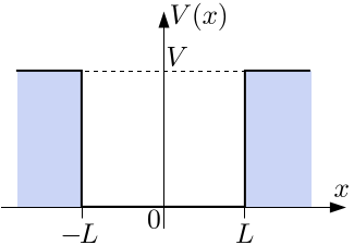
我们已经看到了无限势阱的结果，但这在现实生活中是不可能存在的 - 一个点不可能相对于另一个点具有无限的势能。让我们考虑对称有限势阱，对吧。如果阱以原点为中心，在数学上更容易处理。如前所述，阱内的势能（在-L和L之间）为0，但在阱外，它是一个有限值V（两侧相等）

$V\left(x\right)={\begin{cases}V,\quad x<-L\\0,\quad -L\leq x\leq L\\V,\quad x>L\end{cases}}$

由于井外的势能是有限的，即使电子的势能小于V，电子也可能从井中逃逸（量子隧穿），因此我们预计会看到一个在井边界处不为零的波函数。

让我们将我们的波函数分成三部分，每一侧一部分，井内一部分

$\psi \left(x\right)={\begin{cases}\psi _{1}\left(x\right),&\quad x<-L\\\psi _{2}\left(x\right),&\quad -L\leq x\leq L\\\psi _{3}\left(x\right),&\quad x>L\end{cases}}$

我们将使用薛定谔方程分别求解每个波函数

[一维时间无关薛定谔方程]

$-{\frac {\hbar ^{2}}{2m}}{\frac {d^{2}}{dx^{2}}}\psi \left(x\right)+V(x)\psi =E\psi$

井内

在井内，势能为零，因此我们可以将薛定谔方程改写为：

$-{\frac {\hbar ^{2}}{2m}}{\frac {d^{2}}{dx^{2}}}\psi _{2}\left(x\right)=E\psi _{2}$

重新排列，

${{d^{2}} \over {dx^{2}}}\psi _{2}\left(x\right)=-{{2mE} \over \hbar ^{2}}\psi _{2}\left(x\right)$

回想一下，能量由下式给出

$E\,$	$=T\left(x\right)+V\left(x\right)\,$
	$={{\hbar ^{2}k^{2}} \over {2m}}$

将E代入我们的微分方程得到

${{d^{2}\psi _{2}\left(x\right)} \over {dx^{2}}}=-k^{2}\psi _{2}\left(x\right)$

现在这是一个标准形式的二阶微分方程。通解由下式给出：

[ψ_2的通解]

$\psi _{2}\left(x\right)=A\sin {kx}+B\cos {kx}$

这里的能量是

$E={\frac {k^{2}\hbar ^{2}}{2m}}$

在这个通解中，A 和 B 可以是任何复数，k 可以是任何实数。

井外

我们现在来看波函数ψ₁所在的区域，即左侧区域。井右侧区域将会有相同的推导。对于井左侧的外部区域，由于势能是恒定的，V(x) = V，我们的薛定谔方程变为

$-{\frac {\hbar ^{2}}{2m}}{\frac {d^{2}}{dx^{2}}}\psi _{1}\left(x\right)=(E-V)\psi _{1}$

有两个可能的解集，取决于E 小于 V（粒子束缚在势阱中）还是 E 大于 V（粒子是自由的）。

非束缚态

对于自由粒子，E > V，令

$\kappa ^{2}={\frac {2m(E-V)}{\hbar ^{2}}}$

得到

${\frac {d^{2}}{dx^{2}}}\psi _{1}\left(x\right)=-\kappa ^{2}\psi _{1}$

具有与井内相同的解形式

$\psi _{1}=C\sin(\kappa x)+D\cos(\kappa x)\quad$

束缚态

此分析将首先关注束缚态，其中E-V。令

$\alpha ^{2}={\frac {2m(V-E)}{\hbar ^{2}}}$

得到

${\frac {d^{2}}{dx^{2}}}\psi _{1}\left(x\right)=\alpha ^{2}\psi _{1}\left(x\right)$

其中通解是指数函数

$\psi _{1}\left(x\right)=Fe^{-\alpha x}+Ge^{\alpha x}\,\!$

类似地，对于井外的另一个区域

$\psi _{3}\left(x\right)=He^{-\alpha x}+Ie^{\alpha x}\,\!$

现在，为了找到手头问题的特定解，我们必须指定适当的边界条件，并找到满足这些条件的 *A* 、*B* 、*F* 、*G* 、*H* 和 *I* 的值。

寻找束缚态的波函数

薛定谔方程的解必须是连续的，并且是连续可微的。这些要求是先前推导的微分方程的边界条件。

在这种情况下，有限势阱是对称的，因此可以通过选择定义明确奇偶性的波函数来利用对称性减少必要的计算。

总结前几节

$\psi \left(x\right)={\begin{cases}\psi _{1}\left(x\right),&\quad x<-L\\\psi _{2}\left(x\right),&\quad -L\leq x\leq L\\\psi _{3}\left(x\right),&\quad x>L\end{cases}}$

我们发现了束缚态的波函数，$\psi _{1},\psi _{2}\,\!$ 和 $\psi _{3}\,\!$ 为

$\psi _{1}\left(x\right)=Fe^{-\alpha x}+Ge^{\alpha x}\,\!$

$\psi _{2}\left(x\right)=A\sin(kx)+B\cos(kx)\quad$

$\psi _{3}\left(x\right)=He^{-\alpha x}+Ie^{\alpha x}\,\!$

其中

$k={\frac {\sqrt {2mE}}{\hbar }}$

$\alpha ={\frac {\sqrt {2m(V-E)}}{\hbar }}$

我们看到，当 *x* 趋于 $-\infty$ 时，*F* 项趋于无穷大。同样，当 *x* 趋于 $+\infty$ 时，*I* 项趋于无穷大。由于波函数对于所有 *x* 必须是有限的，这意味着我们必须设置 *F* = *I* = 0，并且我们有

$\psi _{1}\left(x\right)=Ge^{\alpha x}\,\!$

$\psi _{2}\left(x\right)=A\sin(kx)+B\cos(kx)$

$\psi _{3}\left(x\right)=He^{-\alpha x}\,\!$

接下来，我们知道总的 $\psi \,\!$ 函数必须是连续的并且可微的。换句话说，函数的值及其导数必须在分割点匹配。

$\psi _{1}(-L)=\psi _{2}(-L)\,\!$		$\psi _{2}(L)=\psi _{3}(L)\,\!$
${\frac {d\psi _{1}}{dx}}(-L)={\frac {d\psi _{2}}{dx}}(-L)\,\!$		${\frac {d\psi _{2}}{dx}}(L)={\frac {d\psi _{3}}{dx}}(L)\,\!$

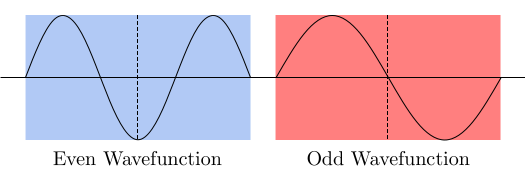
首先，我们需要回顾一下，必须存在具有明确定义的 奇偶性 的波函数解，奇数 **或** 偶数。由于正弦函数是奇函数，余弦函数是偶函数，我们可以寻找阱中正弦或余弦形式的波函数解。现在我们可以分别分析偶数和奇数波函数。将证明对于束缚态，偶数解和奇数解总是具有不同的能量。这意味着没有简并，因此没有束缚本征态是正弦和余弦的线性组合，并且所有束缚态都具有明确定义的奇偶性。下面是一个图，显示了一个偶数奇偶性波函数和一个奇数奇偶性波函数。这些仅用于说明，并不一定与给定问题相关，它们旨在仅传达波函数的对称性。

偶数波函数

偶数解的波函数没有奇数（正弦）分量，所以三个波函数现在是

$\psi _{1}\left(x\right)=Ge^{\alpha x}\,\!$

$\psi _{2}\left(x\right)=B\cos(kx)$

$\psi _{3}\left(x\right)=He^{-\alpha x}\,\!$

现在让我们考虑在两个“连接点”处要求波函数连续的条件

$Ge^{-\alpha L}=B\cos(-kL)\,$

$He^{-\alpha L}=B\cos(kL)\,$

由于余弦函数是偶函数，这两个方程具有相同的右手边。因此我们有

$Ge^{-\alpha L}=He^{-\alpha L}\,$

$G=H\,$

边界处导数连续的条件给了我们以下结果

$\alpha Ge^{-\alpha L}=-kB\sin(-kL)\,$

$\alpha He^{-\alpha L}=kB\sin(kL)\,$

鉴于 G 和 H 相等，我们现在可以将第二条件中的任何方程式除以第一条件中的任何方程式。我将选择每个集合中的第一个方程式。

${\frac {\alpha Ge^{-\alpha L}}{Ge^{-\alpha L}}}={\frac {-kB\sin(-kL)}{B\cos(-kL)}}$

现在我们得到了 α 的表达式（回想一下，tan 函数是奇函数，因此负号相互抵消）。

$\alpha =k\tan \left(kL\right),$

其中

$k={\frac {\sqrt {2mE}}{\hbar }}$

$\alpha ={\frac {\sqrt {2m(V-E)}}{\hbar }}$

这可以简化为以下方程式

${\frac {\alpha }{k}}=\tan \left(kL\right),$

${\sqrt {\frac {V-E}{E}}}=\tan \left({\frac {\sqrt {2mE}}{\hbar }}L\right)$

偶宇称波函数存在于满足此方程式的能量 (E) 处。此方程式非常难以解析求解，但可以很容易地数值求解或图形求解。这将在后面完成。首先，我们将推导出奇宇称波函数。

奇波函数

奇解的波函数没有偶数（余弦）分量，因此三个波函数现在是

$\psi _{1}\left(x\right)=Ge^{\alpha x}\,\!$

$\psi _{2}\left(x\right)=A\sin(kx)$

$\psi _{3}\left(x\right)=He^{-\alpha x}\,\!$

现在让我们考虑在两个“连接点”处要求波函数连续的条件

$Ge^{-\alpha L}=A\sin(-kL)\,$

$-He^{-\alpha L}=A\sin(kL)\,$

由于正弦是奇函数，我们可以看到

$Ge^{-\alpha L}=-He^{-\alpha L}\,$

$G=-H\,$

边界处导数连续的条件给了我们以下结果

$\alpha Ge^{-\alpha L}=kA\cos(-kL)\,$

$\alpha He^{-\alpha L}=kA\cos(kL)\,$

将第二组中的第一个方程式除以第一组中的第一个方程式（任何组合都可以），我们得到

${\frac {\alpha Ge^{-\alpha L}}{Ge^{-\alpha L}}}={\frac {kA\cos(-kL)}{A\sin(-kL)}}$

$\alpha =k\cot \left(-kL\right)\,$

并且因为 cot 是奇函数，

${\frac {\alpha }{k}}=-\cot \left(kL\right)$

${\sqrt {\frac {V-E}{E}}}=-\cot \left({\frac {\sqrt {2mE}}{\hbar }}L\right)$

当能量满足此条件时，存在奇宇称波函数。与偶波函数一样，这个方程不容易解析求解，但可以图形或数值求解。

能级图解法

让我们快速回顾一下我们的目标。我们希望找到电子在有限方势阱中束缚态的能量。当满足以下条件之一时，就会出现能级：

[偶波函数存在条件]

${\frac {\alpha }{k}}=\tan \left(kL\right)$

[奇波函数存在条件]

${\frac {\alpha }{k}}=-\cot \left(kL\right)$

我们可以将三个函数一起绘制在针对能量 *E* 的图形上。条件在交叉点处满足，如下所示。因此，我们可以通过读取交叉点的能量来找到允许的能级。在我们绘制图形之前，我们需要选择系统的一些属性。让我们将阱的宽度设置为 0.4 纳米（*L* = 0.2 纳米），并将势垒 *V* 设置为 75 电子伏特。

我们看到有六个允许的能级：偶波函数大约在 2、17 和 46 电子伏特处，奇波函数大约在 7.5、30 和 64.5 电子伏特处。这种方法提供了一种简单的方法来找出有多少能级以及它们大致位于何处。虽然图解法在理论上与任何方法一样精确，但实际上可以使用纯数值方法获得更高的精度。

还要注意，无论势垒多么小，都将 *始终* 至少存在一个偶解，对应于第一个交点。奇解的存在取决于 V 的值。

能级数值方法

有许多数值方法可用于求解这些方程。虽然这些方程无法精确求解，但它们 *可以* 被微分。这意味着我们可以使用 牛顿-拉夫森 迭代，这些迭代通常收敛速度很快。通过使用图解法对根的位置有一个大致的了解，我们可以为迭代选择合适的起始值。

以下两个方程是使用迭代求解的方程（牛顿-拉夫森方法需要一个等于零的函数）。

${\frac {\alpha }{k}}-\tan \left(kL\right)=0$

${\frac {\alpha }{k}}+\cot \left(kL\right)=0$

迭代需要这些方程的导数（除非由计算机自动完成），如下所示：

${\frac {-V}{2E^{2}{\sqrt {\frac {V-E}{E}}}}}-{\frac {Lm}{\hbar {\sqrt {2mE}}}}\sec ^{2}\left({\frac {L{\sqrt {2mE}}}{\hbar }}\right)$

${\frac {-V}{2E^{2}{\sqrt {\frac {V-E}{E}}}}}-{\frac {Lm}{\hbar {\sqrt {2mE}}}}\csc ^{2}\left({\frac {L{\sqrt {2mE}}}{\hbar }}\right)$

下表显示了该系统中的六个能级、迭代的起始值以及能量（精确到小数点后五位）。

n	宇称	起始值/eV	能量/eV
1	偶	2	1.89660
2	奇	8	7.56592
3	偶	17	16.93946
4	奇	30	29.87241
5	偶	46	46.05440
6	奇	64	64.60181

让我们将这些值与无限方势阱的前六个能级进行比较，我们之前已经了解了如何推导出这些能级。

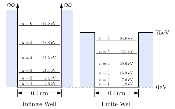
如您所见，有限势阱中的能级低于无限势阱中的能级。这是由于波函数扩展到势阱的边界之外，有效地导致了更大的盒子。由于更大的盒子会导致更低的能级，因此这是合理的。

查找数值波函数

我们找到了评估有限势阱中存在的能级的方法，这通常是唯一需要的的信息，但我们也可以找到波函数的形状。我们已经知道它的近似形状——它在势阱内是正弦形的，并在势阱外呈指数衰减至零。

第一能级

让我们从第一个（最低）能级开始，它是偶数。我们已经定义了波函数的分段如下

$\psi _{1}\left(x\right)=Ge^{\alpha x}\,\!$

$\psi _{2}\left(x\right)=B\cos(kx)$

$\psi _{3}\left(x\right)=He^{-\alpha x}\,\!$

现在我们知道能级，我们可以轻松计算k和α。这意味着我们只需要找到G，B和H。我们已经证明G=H。由于我们之后需要对波函数进行归一化，因此我们可以在此时任意地调整函数的缩放比例而不会造成影响。让我们将B的值设置为1。这样我们只需要找到满足连续边界条件的G（=H）的值。

$\psi _{3}(L)=\psi _{2}(L)\,\!$

$Ge^{-\alpha L}=\cos(kL)\,$

重新排列，

$G={\frac {\cos(kL)}{e^{-\alpha L}}}$

第一能级上的k和α以及E的值

• E = 1.89660eV = 3.03868 × 10^-19 J
• k = 7.05548 × 10⁹
• α= 4.38034 × 10¹⁰

这使得

• G = 1014.31

现在我们可以将波函数相对于位置绘制出来。注意，我们还没有进行归一化，所以单位是任意的。

我们可以看到波函数明显地延伸到经典禁区（蓝色）。如果梯度的精确匹配难以理解，请记住正是这种条件导致了k和α的定义。但是，由于导致这一点的计算仅适用于有效的能量，如果你尝试绘制非有效能量的波函数，你将得到一个连续（因为获取G的方法强制执行这一点）但不是平滑的图形，这意味着该解不适合物理系统。

因为我们没有能量与图形形状之间的简单关系（注意G作为E的相当复杂的函数而改变），我们无法找到一个易于表达的归一化系数。但是，通过积分波函数的平方，我们仍然可以对其进行评估

$\int _{-\infty }^{\infty }|\psi (x)|^{2}dx=1$

$\int _{-\infty }^{-L}|\psi _{1}(x)|^{2}dx+\int _{-L}^{L}|\psi _{2}(x)|^{2}dx+\int _{L}^{\infty }|\psi _{3}(x)|^{2}dx=1$

$\psi _{0}^{2}\left[\int _{-\infty }^{-L}G^{2}e^{2\alpha x}dx+\int _{-L}^{L}\cos ^{2}(kx)dx+\int _{L}^{\infty }G^{2}e^{-2\alpha x}dx\right]=1$

这个积分非常简单，得到以下归一化系数

• ψ₀=66990.6

将此与无限势阱的70710.7进行比较。记住在进行此积分时要考虑单位（通常是纳米会导致问题）。归一化系数在这里较低是有道理的，因为波函数扩展得更远，因此当正弦曲线被缩放为1时，它的面积更大，这意味着它必须乘以更小的数字才能得到在某个地方找到粒子的单位概率。

第二能级

现在让我们考虑第二个能级，它是奇数。波函数由下式给出

$\psi _{1}\left(x\right)=Ge^{\alpha x}\,\!$

$\psi _{2}\left(x\right)=A\sin(kx)$

$\psi _{3}\left(x\right)=He^{-\alpha x}\,\!$

其中G = -H。设置A=1，并继续如上所述，我们得到以下结果

• E = 7.56592eV = 1.21219389 × 10^-18 J
• k = 1.40919 × 10¹⁰
• α= 7.99293 × 10⁹

这使得G为1432.53，并导致以下图形

要获得归一化系数，我们输入

$\int _{-\infty }^{\infty }|\psi (x)|^{2}dx=1$

$\int _{-\infty }^{-L}|\psi _{1}(x)|^{2}dx+\int _{-L}^{L}|\psi _{2}(x)|^{2}dx+\int _{L}^{\infty }|\psi _{3}(x)|^{2}dx=1$

$\psi _{0}^{2}\left[\int _{-\infty }^{-L}G^{2}e^{2\alpha x}dx+\int _{-L}^{L}\sin ^{2}(kx)dx+\int _{L}^{\infty }G^{2}e^{-2\alpha x}dx\right]=1$

这得到一个66849.7的归一化系数。这略小于第一能级的系数。由于波函数进一步扩展到势垒区域（在图形中并不明显，但可以观察到），这是可以预期的。我们可以看到这种模式在所有六个能级中持续存在

n	宇称	G	ψ0
1	偶	1014.31	66990.6
2	奇	1432.53	66849.7
3	偶	-1168.56	66575.5
4	奇	-615.794	66073.7
5	偶	194.185	65055.8
6	奇	25.2653	61954.1

无界状态

对于一个粒子，其能量高于势阱顶部的能量 V，也会有允许的能级。这些能级被称为无束缚态，因为它们在阱外不会衰减到零。但是，它们肯定仍然受势阱的影响。无束缚态也称为连续态，因为与离散的束缚态不同，它们在满足以下条件的连续能量范围内都有解

$E>V\,$

回顾α的定义

$\alpha ={\frac {\sqrt {2m(V-E)}}{\hbar }}$

在无束缚态中，它是虚数，这意味着我们不能使用与束缚态相同的解法。如果你观察图形解，你会发现α/k的线在V处结束，这意味着在此点之后不再有有效的束缚态能级。

我们在本页开头看到，无束缚态在阱外的波函数为

$\psi _{1}\left(x\right)=C\sin(\kappa x)+D\cos(\kappa x)\quad$

其中

$\kappa ={\sqrt {\frac {2m(E-V))}{\hbar ^{2}}}}$

阱内的解与束缚态相同

$\psi _{2}\left(x\right)=A\sin {kx}+B\cos {kx}$

由于势能围绕原点对称，因此对于无束缚态也必须有定义奇偶性的解，因此我们将选择奇波函数和偶波函数的基底。与以前一样，我们知道总波函数必须是连续且可微的。换句话说，函数值及其导数必须在分割点处匹配。

$\psi _{1}(-L)=\psi _{2}(-L)\,\!$		$\psi _{1}(L)=\psi _{2}(L)\,\!$
${\frac {d\psi _{1}}{dx}}(-L)={\frac {d\psi _{2}}{dx}}(-L)\,\!$		${\frac {d\psi _{1}}{dx}}(L)={\frac {d\psi _{2}}{dx}}(L)\,\!$

奇波函数

对于奇波函数，我们可以忽略$\psi _{2}$的余弦项，但不能忽略$\psi _{1}$和$\psi _{3}$

$\psi _{2}\left(x\right)=A\sin {kx}\,\!$

$\psi _{1}\left(x\right)=C\sin {\kappa x}+D\cos {\kappa x}=C\sin {(\kappa x-\phi )}$

$\psi _{3}\left(x\right)=E\sin {\kappa x}+F\cos {\kappa x}=C\sin {(\kappa x+\phi )}$

$\psi _{1}$ 和 $\psi _{3}$ 本身不是奇函数，但对于所有 x 定义的通用函数 $\psi$ 是奇函数，注意到对于任何 $x_{0}>L$

$\psi _{1}\left(-x_{0}\right)=\psi _{3}\left(x_{0}\right)$

应用波函数连续性边界条件，我们得到每个边界处的相同结果。

$C\sin {(\kappa L+\phi )}=A\sin {kL}\,\!$

取导数并在 L 处要求连续性，我们得到

$\kappa C\cos {(\kappa L+\phi )}=kA\cos {kL}\,\!$

选择具有已定义奇偶性的波函数将问题简化为仅在一个点调整波函数及其导数的值（因为另一个点会产生相同的方程）。因此我们有两个方程，三个变量。我们将选择井外波函数的振幅 C 为单位。最后，我们将对整个一维有限井上的 $\psi$ 进行归一化。

用波函数连续性导出的方程除以导数连续性的方程

$\tan {(\kappa L+\phi )}={\frac {\kappa }{k}}\tan {kL}$

$\phi =\arctan {({\frac {\kappa }{k}}\tan {kL}})-\kappa L$

将相位 $\phi$ 代入 L 处的连续性方程，并取 C=1，我们得到

$A={\frac {\sin {(\kappa L+\phi )}}{\sin {kL}}}$

因此我们看到对于任何能量、井深和宽度，都存在奇波函数解。当

$\sin {kL}=0,\!$

时，在井上方存在共振。这类似于光学中的法布里-珀罗共振。

偶数波函数

与奇数波函数相同，我们可以忽略 $\psi _{2}$ 的正弦项，但不能忽略偶数波函数的 $\psi _{1}$ 和 $\psi _{3}$ 的正弦项。

$\psi _{2}\left(x\right)=B\cos {kx}\,\!$

$\psi _{1}\left(x\right)=C\sin {\kappa x}+D\cos {\kappa x}=D\cos {(\kappa x-\phi )}$

$\psi _{3}\left(x\right)=E\sin {\kappa x}+F\cos {\kappa x}=C\cos {(\kappa x+\phi )}$

应用波函数连续性边界条件，我们得到每个边界处的相同结果。

$C\cos {(\kappa L+\phi )}=B\cos {kL}\,\!$

取导数并在 L 处要求连续性，我们得到

$\kappa C\sin {(\kappa L+\phi )}=kA\sin {kL}\,\!$

用波函数连续性导出的方程除以导数连续性的方程

$\tan {(\kappa L+\phi )}={\frac {k}{\kappa }}\tan {kL}$

$\phi =\arctan {({\frac {k}{\kappa }}\tan {kL}})-\kappa L$

将相位 $\phi$ 代入 L 处的连续性方程，并取 C=1，我们得到

$A={\frac {\cos {(\kappa L+\phi )}}{\cos {kL}}}$

因此，我们看到对于任何能量、阱深和宽度，都存在偶数波函数解。当

$\cos {kL}=0,\!$