电路理论/相量/示例/示例 10

用于示例 10 的并联 RL 电路

假设电流源由$I_{s}(t)=120{\sqrt {2}}cos(377t+120^{\circ })$ 定义，求解所有其他电压和电流，并检查功率。

标注回路和节点

用于分析的并联 RL 电路标记图

在并联电路中，所有器件上的电压都完全相同。

已知量、未知量和方程式

已知量：$I_{s},R,L$

未知量：$V_{s},i_{R},i_{L}$

方程式：$V_{s}(t)=R*i_{R}(t),V_{s}=L*{d \over dt}i_{L}(t),i_{R}(t)+i_{L}(t)-I_{s}(t)=0$

相量符号

mupad 尝试进行一些相量代数运算...需要找到一种方法以符号形式求解矩形形式和极坐标形式的实部和虚部，并找到数值评估的方法...m 文件

时域

按顺序评估端子关系

$i_{R}(t)={\frac {V_{s}}{R}}$

$i_{L}(t)=\int {\frac {V_{s}}{L}}dt$

代入这个等式

$I_{s}(t)=i_{R}(t)+i_{L}(t)$

$I_{s}(t)={\frac {V_{s}}{R}}+\int {\frac {V_{s}}{L}}dt$

为了让数学家满意，需要将其转换为微分方程，所以对等式两边求导（不要让他们看到你在这样做）。

${dI_{s}(t) \over dt}={\frac {1}{R}}{dV_{s} \over dt}+{\frac {V_{s}}{L}}$

所以得到了一个可以求解的微分方程 $V_{s}$.

相量域

现在将这两个运算转换为相量域。

${I_{s}}(t)\rightarrow \mathbb {I} _{s}\rightarrow I_{m}\angle \phi$

$V_{s}(t)\rightarrow \mathbb {V} _{s}$

$\int V_{s}(t)dt\rightarrow {\frac {1}{j\omega }}\mathbb {V} _{s}$

所以

$\mathbb {I} _{s}={\frac {\mathbb {V} _{s}}{R}}+{\frac {\mathbb {V} _{s}}{j\omega L}}$ 或 $j\omega \mathbb {I} _{s}=j\omega {\frac {\mathbb {V} _{s}}{R}}+{\frac {\mathbb {V} _{s}}{L}}$

求解 $\mathbb {V} _{s}$

$\mathbb {V} _{s}={\frac {\mathbb {I} _{s}j\omega LR}{R+j\omega L}}$

转换为矩形形式

$\mathbb {V} _{s}=\mathbb {I} _{s}*{\frac {\omega ^{2}L^{2}R+j\omega LR^{2}}{R^{2}+\omega ^{2}L^{2}}}$

转换为极坐标形式

$\mathbb {V} _{s}=\mathbb {I} _{s}{\frac {\sqrt {(\omega ^{2}L^{2}R)^{2}+(\omega LR^{2})^{2}}}{R^{2}+\omega ^{2}L^{2}}}\angle \arctan({\frac {R}{\omega L}})$

回到时域

$V_{s}(t)=I_{m}{\frac {\sqrt {(\omega ^{2}L^{2}R)^{2}+(\omega LR^{2})^{2}}}{R^{2}+\omega ^{2}L^{2}}}\cos(\phi +\arctan({\frac {R}{\omega L}}))$

会存在一个积分常数，但现在无法计算。

这是从一个微分方程推导出的。

在将齐次解添加到上述特解后，将计算积分常数。

相量数值解

相量数值解将所有相量组合成矩形形式，然后直接转为极坐标形式。角度位于第三象限... m-文件

时域

按顺序评估端子关系

$i_{R}(t)={\frac {V_{s}}{10}}$

$i_{L}(t)=\int {\frac {V_{s}}{.01}}dt$

代入这个等式

$I_{s}(t)=i_{R}(t)+i_{L}(t)$

因此得到一个关于 $V_{s}$ 的微分方程，可以求解。

$I_{s}(t)={\frac {V_{s}}{10}}+\int {\frac {V_{s}}{.01}}dt$

相量域

将此代入从相量分析得到的符号时域解... 角度相同，位于第三象限... 这次为正数 ... m-文件

选择在时域进行计算

回到时域

$V_{s}(t)=120*{\sqrt {2}}{\frac {\sqrt {(377^{2}*.01^{2}*10)^{2}+(377*.01*10^{2})^{2}}}{10^{2}+377^{2}*.01^{2}}}\cos(377t+{\frac {2*\pi }{3}}+\arctan({\frac {10}{377*.01}}))$

$V_{s}(t)=599\cos(377t+3.30)$

$i_{R}(t)=59.9\cos(377t+3.30)$

$i_{L}(t)=159\sin(377t+3.30)=159\cos(377t+1.74)$

拉普拉斯符号

时域

按顺序评估端子关系

$i_{R}(t)={\frac {V_{s}}{R}}$

$i_{L}(t)=\int {\frac {V_{s}}{L}}dt$

代入这个等式

$I_{s}(t)=i_{R}(t)+i_{L}(t)$

因此得到一个关于 $V_{s}$ 的微分方程，可以求解。

$I_{s}(t)={\frac {V_{s}}{R}}+\int {\frac {V_{s}}{L}}dt$

拉普拉斯域

现在将两者都转换为拉普拉斯域..

${I_{s}}(t)\rightarrow {\mathcal {L}}\left\{{I_{s}}(t)\right\}$

$V_{s}(t)\rightarrow {\mathcal {L}}\left\{V_{s}(t)\right\}$

$\int V_{s}(t)dt\rightarrow {\frac {1}{s}}{\mathcal {L}}\left\{V_{s}(t)\right\}\$

所以

${\mathcal {L}}\left\{{I_{s}}(t)\right\}={\frac {{\mathcal {L}}\left\{V_{s}(t)\right\}}{R}}+{\frac {{\mathcal {L}}\left\{V_{s}(t)\right\}}{sL}}$

求解${\mathcal {L}}\left\{V_{s}(t)\right\}$

${\mathcal {L}}\left\{V_{s}(t)\right\}=$${\frac {{{\mathcal {L}}\left\{{I_{s}}(t)\right\}}LsR}{R+sL}}$

此时拉普拉斯符号解必须停止。下一步取决于${{\mathcal {L}}\left\{{I_{s}}(t)\right\}}$的形式。

回到时域

在没有${{\mathcal {L}}\left\{{I_{s}}(t)\right\}}$的情况下，这是无法完成的。函数${{\mathcal {L}}\left\{{I_{s}}(t)\right\}}$的形式决定了逆映射。

拉普拉斯数值

拉普拉斯解法与之前一样存在相同的问题...常数...正弦项符号错误 m 文件

时域

$I_{s}(t)=120{\sqrt {2}}cos(377t+2.09)$

$R=10$

$L=.01$

拉普拉斯域

${I_{s}}(t)\rightarrow {\mathcal {L}}\left\{{I_{s}}(t)\right\}={\mathcal {L}}\left\{120{\sqrt {2}}cos(377t+120^{\circ })\right\}=-{\frac {(170.0*(0.5*s+326.0))}{(s^{2}+142129)}}$

${\mathcal {L}}\left\{V_{s}(t)\right\}={\frac {\frac {-17.0*s*(0.5*s+326.0)}{(s^{2}+142129)}}{10+.01*s}}$

时域

$V_{s}(t)={\mathcal {L}}^{-1}\left\{i(t)\right\}=(-2.58)*e^{-{\frac {t}{.001}}}+97.2sin(377t)-591cos(377*t)$

答案比较

$V_{s}(t)=599\cos(377t-2.98)$ ... 来自相量域的数值解

$V_{s}(t)=599\cos(377t+3.30)$ ... 将其代入符号时域的解

相位角在第三象限的位置完全相同。

仿真

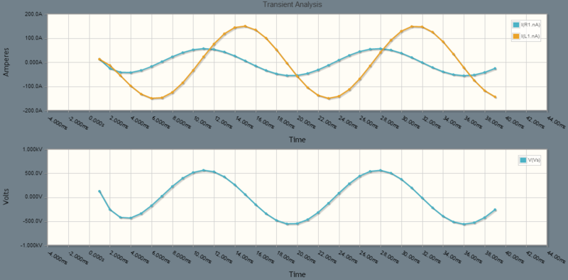
$i_{r}$ 与 $V_{s}$ 同相，正如预期的那样。 $V_{s}$ 超前于 $i_{L}$（通过电感）${\frac {\pi }{2}}$，正如预期的那样。一切似乎都围绕着 0 伏特，因此没有常数在起作用。

周期检查

上面的周期看起来介于 16ms 和 17ms 之间，更接近 17ms。这与公式一致

$\omega =2\pi *f$

$f={\frac {\omega }{2\pi }}$

$T={\frac {1}{f}}={\frac {2\pi }{\omega }}={\frac {2\pi }{377}}=16.7ms$

幅值检查

V_s 的幅值超过 500 伏特……虽然可能不到 600 伏特。

暂态响应检查

一切都从零开始。这意味着只有仿真窗口的中间到右侧才能显示我们可以与计算值进行比较的稳态信息。

相位检查

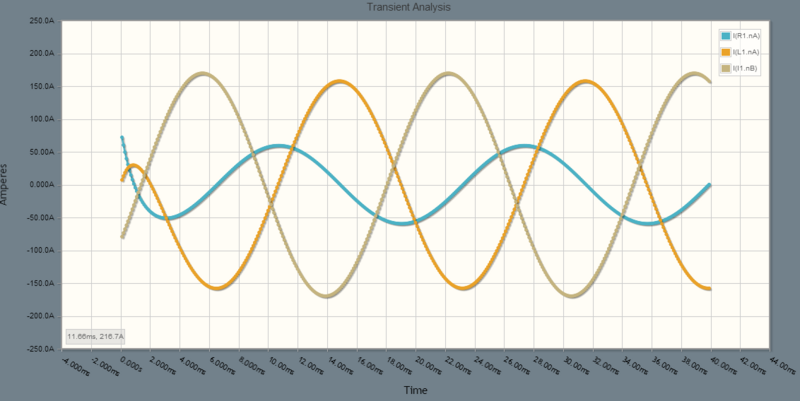
$I_{s}$（棕色）、$i_{R}$（蓝色，与源电压同相）、以及 $i_{L}$（橙色）。$i_{R}V_{s}$（蓝色）超前于 $i_{L}$（橙色）${\frac {\pi }{2}}$。棕色电流（起点）在 2.09 弧度处为起点。蓝色电流应该比棕色电流超前 3.30-2.09=1.21 弧度，即 69.3 度，大约为 3.21 毫秒，或比棕色电流高出 1.5 个方格。在仿真软件处理初始能量失衡的开始阶段看不到这一点，但在仿真中期，蓝色电流比棕色电流超前约 1.5 个方格。所以一切正常。

功率分析

常数将为这种分析增加一些直流功率或有功功率。在不知道它们是什么的情况下，我们无法计算出它们的影响。因此，现在我们坚持使用相量域功率分析。

$\mathbb {I} _{s}=120{\sqrt {2}}\angle 2.09$

$\mathbb {V} _{s}=599\angle 3.30$

$\mathbb {I} _{s}^{*}=120{\sqrt {2}}\angle -2.09$

如果 :$\mathbb {V} =M_{v}\angle \phi _{v}\quad$, 以及 $\quad \mathbb {I} =M_{i}\angle \phi _{i}$ 那么

$\mathbb {S} =\mathbb {V} \mathbb {I} ^{*}={\frac {M_{v}M_{i}}{2}}\angle (\phi _{v}-\phi _{i})={\frac {120{\sqrt {2}}*599}{2}}\angle (3.30-2.09)=10,164\angle 1.21=3,586+9,510j$

以及

$cos(1.21)=.357$

这是一个糟糕的功率因数。低于 0.9 的功率因数会导致您收到电力公司的访问，或者电线杆上的变压器可能会炸毁。公用事业的视在功率远大于客户愿意支付的功率。

值	单位	描述
$10,164$	伏安 va	视在功率，电力公司管理的功率：他们设计的峰值功率，他们必须提供的峰值功率
$.357$	无量纲	功率因数，有功功率与视在功率的比值，理想值为 1
$3,590$	瓦特 W	有功功率、平均功率、有效功率...消费者愿意支付的功率（瓦特小时）
$9,510$	无功功率 var	无功功率...为什么房间里的不是所有插座都在同一个断路器上

直觉

应该有一个方法可以在 mupad 中以符号形式进行相量数学...可能使用矩阵。